SUBSAMPLE keyword
SUBSAMPLE reduces the number of rows in a query result while preserving the
visual shape of the data. It selects the most representative points from a
time-ordered dataset, making it ideal for rendering charts at screen resolution
without transferring millions of rows to the client. One method, sdt,
reduces rows to within a value tolerance instead of to a row budget, which
suits error-bounded telemetry compression.
Unlike SAMPLE BY, which computes new aggregate
values at synthetic bucket boundaries, SUBSAMPLE selects rows from its
immediate query input and never alters their values. Over a direct table
scan, every output row is a physical table row with its original timestamp,
so output timestamps can be used in joins and users can drill down to the
exact source record behind any point on a chart. After SAMPLE BY,
GROUP BY, a join, or a computed projection, the selected rows are the
derived rows of that query, which can carry aggregate values or synthetic
timestamps.
The query source must provide a
designated timestamp, and the SELECT
list must preserve it. A table with a designated timestamp is not enough if
the projection omits that column or replaces it with an expression that loses
the designation.
Every method is also available as a window function that returns a keep flag for each row instead of the reduced row set. See window-function form.
Syntax
SELECT columns
FROM table
[WHERE conditions]
[LATEST ON ...]
[SAMPLE BY ... | GROUP BY ...]
[WINDOW ...]
SUBSAMPLE method(arguments)
[ORDER BY ...]
[LIMIT ...]
SUBSAMPLE goes after the WHERE, LATEST ON, SAMPLE BY, GROUP BY,
and WINDOW clauses, and before ORDER BY and LIMIT. The SELECT list
must include the designated timestamp, and for the value-based and
tolerance-based methods it must also include valueColumn.
method(arguments) is one of:
SUBSAMPLE lttb(valueColumn, targetPoints [, gapThreshold])
SUBSAMPLE { m4 | minmax }(valueColumn, targetPoints)
SUBSAMPLE uniform(targetPoints)
SUBSAMPLE cadence(stride [, seed])
SUBSAMPLE sdt(valueColumn, compdev)
sdt cannot share a query level with SAMPLE BY, GROUP BY, DISTINCT,
or a join. See query shape restrictions.
Where:
valueColumn- the numeric column used to decide which points are visually significant. Required forlttb,m4,minmax, andsdt. Not used byuniformorcadence.targetPoints- target number of output rows. Supports integer literals, DECLARE variables, and bind variables ($1). Must be at least 2. Maximum is 2,147,483,647.stride- (cadenceonly) step distance between emitted rows. This is not an output count:cadence(500)emits one row out of every 500.seed- (cadenceonly) optional integer seed orNULL. See cadence.gapThreshold- (lttbonly) optional interval that enables gap-preserving mode. See gap-preserving LTTB.compdev- (sdtonly) the compression deviation: a constant, finite, non-negative error tolerance in the units ofvalueColumn. This is not an output count: the data decides how many rowssdtretains. See sdt.
Execution order
SUBSAMPLE runs after SAMPLE BY, GROUP BY, and window functions, but
before ORDER BY and LIMIT. All value computations are complete before
downsampling decides which rows to keep, and a final ORDER BY or LIMIT
operates on the selected rows. SUBSAMPLE only selects rows. It never
modifies computed values.
Internally, SUBSAMPLE computes a keep-or-drop flag for every input row,
the same way a window function computes one value per row, and then filters
the input down to the flagged rows. This selection stage makes two passes
over its input and runs serially. It does not block upstream parallel
execution. For example, a parallel SAMPLE BY completes before SUBSAMPLE
reads its output.
Output order
Every algorithm computes its selection against an ascending
designated-timestamp traversal of the input, but the query returns the
selected rows in the order of the incoming query. A descending timestamp
input stays descending, and an input explicitly ordered by another column
keeps that order. Add a final ORDER BY when you need a specific output
order.
Supported value types
The value column of lttb, m4, and minmax must be a numeric type:
DOUBLE, FLOAT, INT, LONG, SHORT, or BYTE. For these three
methods, a row is not eligible for selection when its value is NULL or
non-finite, or when its timestamp is NULL. Rows skipped this way still
count toward the input row limit.
The value column of sdt accepts the same numeric types and is compared as
DOUBLE. Unlike the three methods above, sdt does not skip a NULL or
non-finite value. It retains that row as a run boundary. See
NULLs and run boundaries.
uniform and cadence take no value column. NULL values in any projected
column do not prevent a row from being selected.
Algorithms
Six algorithms are available. The first three (lttb, minmax, m4)
inspect values to decide which rows are visually significant. The next two
(uniform, cadence) ignore values and select rows purely by position.
They are useful when the input is dense or as a baseline. The last one
(sdt) also inspects values, but takes an error tolerance instead of a
target row count or a stride, so the data decides how many rows it keeps.
All six select existing rows from their input. No values are ever interpolated or computed. The diagrams below use a 24-point series as input (think 24 hourly bars over one day):

lttb - Largest Triangle Three Buckets
Divides the data into equal-sized row-count buckets and selects the point in each bucket that forms the largest triangle with its neighbors. The idea is that points where the line changes direction sharply (a spike, a valley, a sudden trend shift) form large triangles and get kept, while points in the middle of a smooth trend form small triangles and get dropped. The first and last points are always kept. Output is exactly N points when at least N eligible rows exist. With fewer eligible rows, all of them are returned.
Best for line charts where the visual shape matters most - a chart drawn from the LTTB output looks nearly identical to one drawn from the full dataset, despite using far fewer points.

How it works:
- First and last points are always selected.
- Remaining data is divided into N-2 equal-sized buckets by row count.
- For each bucket, the point creating the largest triangle area with the previously selected point and the average of the next bucket is chosen.
When the input is much larger than the target (more than about 8 eligible rows per target point), QuestDB uses a two-stage variant known as MinMaxLTTB. It first preselects the local minima and maxima from row-count bins, then runs the triangle stage on those candidates only. The output count is the same, but the selected points can differ from classic LTTB run over every raw row. Smaller inputs use classic LTTB directly.
SELECT timestamp, avg(price) avg_price
FROM fx_trades
WHERE symbol = 'EURUSD'
  AND timestamp IN '$today'
SAMPLE BY 1h
SUBSAMPLE lttb(avg_price, 8)
Gap-preserving LTTB
Standard LTTB divides data by row count, so it connects across time gaps. An optional third parameter sets a gap threshold:
SUBSAMPLE lttb(price, 12, '6h')
When specified, LTTB scans for gaps where consecutive timestamps are further apart than the threshold. Gaps below the threshold are ignored - the data is treated as continuous. Gaps above the threshold split the data into separate segments, each downsampled independently. Each segment receives an integer share of the target proportional to its row count, with a minimum of two points (one for a single-row segment) so that a multi-row segment keeps its endpoints.
The diagrams below show a dataset with two gaps - a small one (3 hours) and a large one (24 hours):

Without gap detection, LTTB treats all points as continuous and connects across both gaps:

With a threshold of '6h', the small gap (3h) is below the threshold so
segments A and B are treated as continuous. The large gap (24h) exceeds the
threshold, so segment C is downsampled separately and both edges of the gap
are retained:

The diagram draws each segment as a separate line, which is what a client
that breaks lines on large timestamp gaps would render. The SQL result
itself is a flat list of rows with no NULL separator row and no segment
identifier, so a renderer that connects consecutive points still joins the
last point of one segment to the first point of the next. To show the
discontinuity on a chart, apply a timestamp-gap or segment-breaking rule in
the client.
Supported interval units: s (seconds), m (minutes), h (hours),
d (days).
Examples: '30s', '5m', '1h', '7d'
SELECT timestamp, price
FROM fx_trades
WHERE symbol = 'EURUSD'
SUBSAMPLE lttb(price, 12, '6h')
Gap-preserving LTTB treats targetPoints as a goal, not an exact count.
Integer rounding of the proportional shares can leave part of the target
unused, so the output can be below targetPoints. When many segments are
detected, the per-segment minimum can push the total output above
targetPoints. This is by design so that the same query does not fail for
one time range and succeed for another. Non-gap LTTB, M4, and MinMax treat
targetPoints as a hard maximum.
minmax - Min/Max per time interval
Divides the time range into equal time intervals and selects up to 2 points per interval: the row with the minimum value and the row with the maximum value. This creates a visual envelope - at any point on the chart, you can see the full range the data covered during that interval. The minimum and maximum rows of every non-empty interval are always retained, and when both resolve to the same row it is emitted once.
Empty intervals emit no rows, so the result retains the absence of samples in those intervals. That alone does not make a line renderer break the line across the gap. As with gap-preserving LTTB, the client must apply a timestamp-gap rule to show the discontinuity.

How it works:
- The total time range is divided into N/2 equal time intervals.
- For each interval, up to 2 points are selected: min, max.
- Duplicate points are removed (if min and max are the same row).
- Empty intervals produce no output.
Output is up to N points (N/2 buckets, up to 2 points each).
SELECT timestamp, avg(price) avg_price
FROM fx_trades
WHERE symbol = 'EURUSD'
  AND timestamp IN '$today'
SAMPLE BY 1h
SUBSAMPLE minmax(avg_price, 8)
m4 - Min/Max/First/Last per time interval
Builds on MinMax by also capturing the first and last rows in each time interval. Where MinMax shows you the range of values in a bucket, M4 also shows you where the data entered and exited - the opening and closing levels. This matters when trends within a bucket are important: a price that opens high, dips, then recovers looks different from one that opens low and climbs. MinMax would show the same min/max range for both; M4 distinguishes them.
Empty intervals emit no rows, with the same rendering caveat as MinMax and gap-preserving LTTB: a line renderer can still bridge the gap unless the client breaks the line.

How it works:
- The total time range is divided into N/4 equal time intervals.
- For each interval, up to 4 points are selected: first, last, min, max.
- When multiple roles resolve to the same physical row (e.g., the minimum value is also the first row), duplicates are removed. A bucket emits between 1 and 4 rows depending on the data.
- Empty intervals produce no output.
Output is up to N points (N/4 buckets, up to 4 points each). In the diagram above, compare the right side with MinMax: M4 captures the exit at i=23 (the pullback after the late spike), while MinMax ends at the peak. M4 gives a more faithful picture of where the data actually settled.
SELECT timestamp, avg(price) avg_price
FROM fx_trades
WHERE symbol = 'EURUSD'
  AND timestamp IN '$today'
SAMPLE BY 1h
SUBSAMPLE m4(avg_price, 8)
targetPoints is a row budget, not a bucket count: N/4 gives the number of
time buckets. SUBSAMPLE m4(col, 1920) creates 480 time buckets and returns
up to 1,920 rows. For one time bucket per pixel column on a 1920-pixel-wide
chart, use SUBSAMPLE m4(col, 7680). Empty buckets and role deduplication
can reduce the returned row count.
uniform - Evenly spaced rows
Selects a target number of rows spaced evenly across the input. First and
last rows are always kept, interior rows are picked at regular positions
between them. Unlike the previous algorithms, uniform does not inspect
values. It reduces row count purely by position in the timestamp-ordered
traversal of the input.
Use uniform when the input is dense and you care about reducing transfer
size more than preserving spikes or troughs. Because it ignores values, it
can visibly miss spikes and troughs. For a line chart where visual fidelity
matters, lttb or m4 produce better results at the same target count.
uniform fits a heatmap, scatter plot, or tabular display where every row
looks similar. It avoids value inspection and the timestamp/value buffer of
the value-based methods, but full-query performance depends on the
surrounding plan.

How it works:
- The first and last rows in timestamp order are always selected.
- Remaining
targetPoints - 2rows are selected at evenly spaced positions between first and last. Fractional positions round half up, so the selection is deterministic. - Output is exactly
targetPointsrows when the input is larger than the target, otherwise all input rows are returned unchanged.
SELECT timestamp, price
FROM fx_trades
WHERE symbol = 'EURUSD'
SUBSAMPLE uniform(500)
cadence - Every Nth row
Selects one row out of every N, starting from a configurable offset. Like
uniform, cadence does not inspect values. It reduces row count by
stepping through the timestamp-ordered traversal of the input at a fixed
rhythm. An optional second parameter
sets the starting offset, either as a fixed seed for reproducible results or
as NULL for a fresh random offset each run.
The stride parameter is the step distance, not the output count. To keep
500 rows, use uniform(500) or lttb(col, 500). cadence(500) emits one
row out of every 500, which is a different (and input-dependent) number.

How it works:
- When
strideis greater than 1 and no larger than the input row count, the first and last rows in timestamp order are always selected. - Between them, one row is selected every
striderows, starting from the offset position. cadence(1)returns every row.- When
strideexceeds the input row count, only the first row is selected. The last row is not pinned in this case.
| Form | Behavior |
|---|---|
cadence(N) | Every Nth row, deterministic, offset 0 |
cadence(N, seed) | Random offset in [0, N), reproducible given seed |
cadence(N, NULL) | Random offset in [0, N), fresh each run |
The seeded and NULL forms exist to avoid phase-lock with periodic signals. If the input has a 1000-row period and you stride by 1000 with offset 0, every emitted row hits the same phase of the period and the chart loses the periodic structure. A random offset breaks this alignment.
Randomizing the offset helps with aliasing on periodic signals, but it does
not make cadence a statistical sampler. It does not produce unbiased
estimates of aggregates like mean or percentile. For those, use
SAMPLE BY with the appropriate aggregate
function.
SELECT timestamp, price
FROM fx_trades
WHERE symbol = 'EURUSD'
SUBSAMPLE cadence(1000)
SELECT timestamp, price
FROM fx_trades
WHERE symbol = 'EURUSD'
SUBSAMPLE cadence(1000, 42)
sdt - Swinging Door Trending
Swinging Door Trending (SDT) is an error-bounded compression method. It
replaces a run of samples with a smaller set of retained samples whose
connecting line approximates the original values within a known bound.
Instead of a target row count or a stride, you supply compdev, short for
compression deviation, a tolerance in the units of the value column, and the
data decides how many rows are retained. A flat signal keeps few rows. A noisy signal, or a smaller
tolerance, keeps more.
SDT suits historian, telemetry, and industrial-sensor workloads, where the acceptable error is known in engineering units (for example, half a degree) and the right number of points is not.

On the same 24-point series, sdt with compdev = 0.05 retains 10 rows.
That count was not requested: it is what the tolerance allows on this data.
Near-straight stretches, such as the climb from i=0 to i=4 and the recovery from
i=16 to i=22, collapse to their two endpoints, while the sharp turns around
the spike keep more points. Unlike minmax and m4, sdt does not pin
extremes. The trough at i=15 is dropped because the line from i=14 to i=16
stays within 2 * compdev of it.
How it works:
- The first eligible sample is retained and becomes the current anchor.
- Each later eligible sample constrains a lower and an upper permissible
slope from that anchor,
compdevbelow and above the sample. - The intersection of those slope constraints forms a narrowing corridor, the swinging door.
- When a new sample makes the corridor empty, the previous eligible sample is retained and becomes the next anchor.
- Processing resumes from the new anchor.
- The final eligible sample is retained when the input ends.
The animation below steps through the mechanism on a separate 20-sample
series with compdev = 0.05. It retains 5 samples (0, 6, 8, 14, and 19),
and the reconstruction error is bounded by 2 * compdev = 0.10.
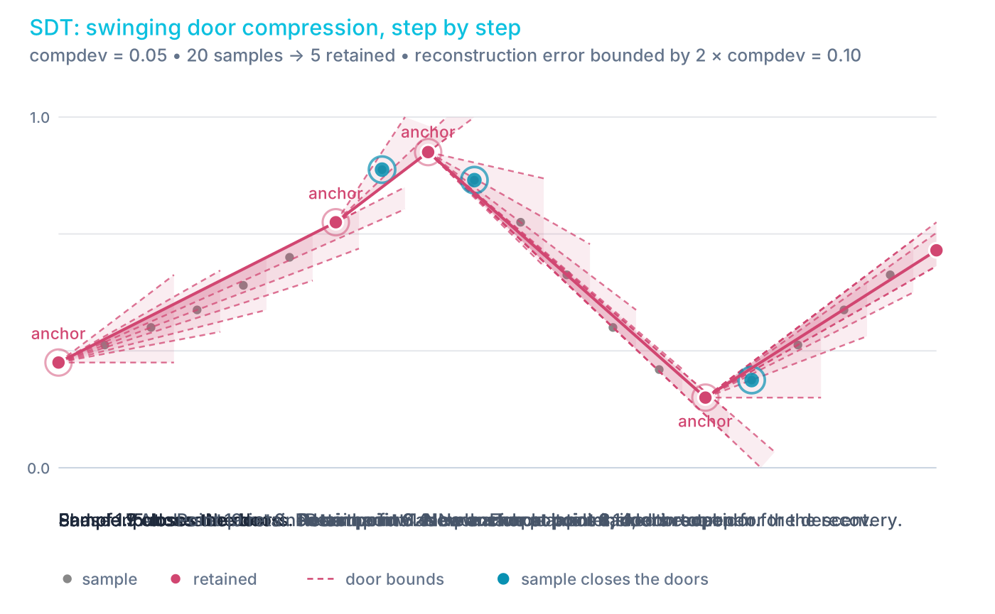
In the animation, the corridor closes when samples 7, 9, and 15 arrive, so samples 6, 8, and 14 are retained. Sample 19 is retained because the input ends there, not because a corridor closed.
SELECT ts, temperature, device_id
FROM sensor_readings
SUBSAMPLE sdt(temperature, 0.5);
SELECT timestamp, price
FROM fx_trades
WHERE symbol = 'EURUSD'
  AND timestamp IN '$today'
SUBSAMPLE sdt(price, 0.0001)
The compdev tolerance
compdev means compression deviation. It is the value-domain tolerance
that sdt uses to constrain the swinging-door corridor. Because the
retained endpoints are original samples, the end-to-end reconstruction bound
is 2 * compdev. See error guarantee.
compdevmust be a constant, finite, non-negative numeric expression. A numeric literal is the normal form. A constant expression such asabs(-0.5)and a DECLARE variable holding a constant also work.- Bind variables and row-dependent expressions, such as a column reference, are rejected.
- A negative,
NULL,NaN, or infinitecompdevis invalid. compdev = 0retains a point whenever finite-precision arithmetic finds a departure from exact collinearity. It is not lossless compression of arbitrary floating-point input.valueColumnmust be a numeric column that appears directly in theSELECTlist.
compdev controls fidelity, not row count. The output count is
data-dependent and there is no way to request a fixed number of points from
sdt. When you need a row budget, use lttb, m4, minmax, or uniform.
Error guarantee
For finite values and strictly increasing timestamps within an SDT run,
linear interpolation between consecutive retained samples differs from every
original eligible sample in that run by no more than 2 * compdev, apart
from normal floating-point rounding.
The bound is 2 * compdev, not compdev. The corridor extends compdev on
each side, and the retained endpoints are original samples rather than
points shifted to the center of the corridor. With compdev = 0.05, the
maximum reconstruction error is 0.10. To guarantee a maximum error of E,
use compdev = E / 2.
Comparisons are conservative in floating-point arithmetic. Near a numerical
boundary, sdt can retain an extra point rather than risk violating the
bound.
NULLs and run boundaries
sdt handles ineligible values differently from lttb, m4, and minmax,
which skip them:
- A row with a
NULLor non-finite value is a hard boundary, and the row itself is retained. - The last eligible sample before the boundary is retained, as it would be at the end of the input.
- The next eligible finite row starts a new run with a fresh anchor.
- A
NULLdesignated timestamp also interrupts normal processing of finite samples.
The error guarantee applies within each run.
Timestamp gaps
A timestamp gap on its own is not a boundary. sdt uses the actual
timestamp distance in its slope calculations, so a long gap influences which
points the corridor retains, but sdt does not promise to retain both sides
of the gap. The result contains no NULL separator row and no segment
identifier. As with
gap-preserving LTTB, a chart that must show a
discontinuity needs a timestamp-gap rule in the client.
The example below has 41 samples at positions 0 to 19 and 40 to 60, with no data in between:
(0, 0.50), (1, 0.55), (2, 0.60), (3, 0.65), (4, 0.70),
(5, 0.95), (6, 0.85), (7, 0.70), (8, 0.60), (9, 0.55),
(10, 0.50), (11, 0.45), (12, 0.40), (13, 0.35), (14, 0.28),
(15, 0.20), (16, 0.25), (17, 0.30), (18, 0.35), (19, 0.40),
(40, 0.45), (41, 0.50), (42, 0.55), (43, 0.58), (44, 0.60),
(45, 0.65), (46, 0.70), (47, 0.75), (48, 0.70), (49, 0.55),
(50, 0.40), (51, 0.25), (52, 0.15), (53, 0.25), (54, 0.40),
(55, 0.55), (56, 0.60), (57, 0.62), (58, 0.60), (59, 0.58),
(60, 0.55)
With compdev = 0.05, sdt retains 11 rows:
(0, 0.50), (4, 0.70), (5, 0.95), (9, 0.55), (15, 0.20),
(19, 0.40), (42, 0.55), (48, 0.70), (52, 0.15), (56, 0.60),
(60, 0.55)

The jump from 19 to 40 does not create a boundary. Sample 19 is retained
because the corridor closes when sample 40 arrives, and sample 40 itself is
not retained: the first retained row after the gap is 42. The largest
reconstruction error in this example is 0.087, at sample 40. That is above
compdev and within the 2 * compdev = 0.10 bound.
Query shape restrictions
sdt accepts a narrower set of query shapes than the other five methods.
It is rejected when the same query level contains:
- aggregate functions or
GROUP BY SAMPLE BYDISTINCT- a join
Filters with WHERE, additional plain columns in the SELECT list, and a
final ORDER BY or LIMIT are all supported. To apply sdt to aggregated
data, compute the aggregation in a subquery or CTE and apply sdt outside
it:
WITH bars AS (
  SELECT timestamp, avg(price) avg_price
  FROM fx_trades
  WHERE symbol = 'EURUSD'
    AND timestamp IN '$today'
  SAMPLE BY 1m
)
SELECT timestamp, avg_price
FROM bars
SUBSAMPLE sdt(avg_price, 0.0001)
The clause form treats its input as a single series. To compress several
series independently in one query, use the
sdt() window function
with PARTITION BY.
Algorithm comparison
| Property | lttb | minmax | m4 | uniform | cadence | sdt |
|---|---|---|---|---|---|---|
| Parameter | targetPoints | targetPoints | targetPoints | targetPoints | stride | compdev (value tolerance) |
| Inspects values | Yes | Yes | Yes | No | No | Yes, as DOUBLE |
| Bucket type | Equal row count | Equal time intervals | Equal time intervals | Equal row spacing | Fixed row stride | None: adaptive swinging corridor |
| Points per bucket | Exactly 1 | Up to 2 (min, max) | Up to 4 (first, last, min, max) | N/A | N/A | N/A |
| Output count | Exactly N when N or more eligible rows exist, otherwise all eligible rows. Gap mode can return fewer or more than N | Up to N | Up to N | Exactly N (or all rows if fewer) | ~rowCount/stride | Data-dependent, no target |
| Error bound | None | None | None | None | None | Linear reconstruction within 2 * compdev, for finite values with strictly increasing timestamps |
| Gap handling | Connects across. With a threshold, segments are selected independently; a line renderer may still bridge the gap | Empty buckets emit no rows; a line renderer may still bridge the gap | Empty buckets emit no rows; a line renderer may still bridge the gap | Connects across | Connects across | A gap is not a boundary and both sides are not guaranteed; no automatic visual break |
NULL values | Skipped | Skipped | Skipped | Not inspected | Not inspected | Retained as run boundaries |
| Best use case | Line charts | Value range overview | Dashboards, SLA | Dense uniform data | Decimation, anti-aliasing | Error-bounded telemetry and historian compression |
| Row limit applies | Yes | Yes | Yes | Yes | Yes | No |
Examples
Chart-ready downsampling
SELECT timestamp, price
FROM fx_trades
WHERE symbol = 'EURUSD'
SUBSAMPLE lttb(price, 500)
SELECT timestamp, price
FROM fx_trades
WHERE symbol = 'EURUSD'
SUBSAMPLE lttb(price, 500, '1h')
SELECT timestamp, price
FROM fx_trades
WHERE symbol = 'EURUSD'
SUBSAMPLE m4(price, 1920)
SELECT timestamp, price
FROM fx_trades
WHERE symbol = 'EURUSD'
SUBSAMPLE minmax(price, 500)
SELECT timestamp, price
FROM fx_trades
WHERE symbol = 'EURUSD'
SUBSAMPLE uniform(500)
SELECT timestamp, price
FROM fx_trades
WHERE symbol = 'EURUSD'
SUBSAMPLE cadence(1000)
SELECT timestamp, price
FROM fx_trades
WHERE symbol = 'EURUSD'
SUBSAMPLE sdt(price, 0.0001)
Composing with SAMPLE BY
SELECT timestamp, avg(price) avg_price
FROM fx_trades
WHERE symbol = 'EURUSD'
SAMPLE BY 1m
SUBSAMPLE lttb(avg_price, 500)
SAMPLE BY computes aggregate values at bucket boundaries. SUBSAMPLE then
selects the most representative rows from that output. The two operations
complement each other: aggregate first, then reduce for display.
sdt cannot share a query level with SAMPLE BY. Put the aggregation in a
subquery or CTE, as shown in
query shape restrictions.
Multiple columns pass through
Because SUBSAMPLE selects existing rows rather than computing new ones,
every selected row retains all the values of its immediate input row. The
query below reads directly from a table, so although side and quantity
are not involved in the downsampling decision, each output row is a trade
with the side and quantity recorded at that timestamp. When the input is an
aggregation, a join, or a computed projection, the pass-through values are
those of the derived row, not of a physical source record.
SELECT timestamp, symbol, side, price, quantity
FROM fx_trades
WHERE symbol = 'GBPUSD'
SUBSAMPLE lttb(price, 500)
After window functions
SELECT timestamp, price,
    avg(price) OVER (ROWS 10 PRECEDING) ma
FROM fx_trades
WHERE symbol = 'EURUSD'
SUBSAMPLE lttb(price, 500)
Window functions compute on the full dataset. SUBSAMPLE then selects from
the result, so the moving average values are accurate.
With DECLARE variable
DECLARE @points := 500
SELECT timestamp, price
FROM fx_trades
WHERE symbol = 'EURUSD'
SUBSAMPLE lttb(price, @points)
With bind variable
SELECT timestamp, price
FROM fx_trades
WHERE symbol = 'EURUSD'
SUBSAMPLE lttb(price, $1)
With ORDER BY and LIMIT
SELECT timestamp, price
FROM fx_trades
WHERE symbol = 'EURUSD'
SUBSAMPLE lttb(price, 100)
ORDER BY price DESC
LIMIT 10
Inside subqueries
SELECT count() FROM (
    SELECT timestamp, price
    FROM fx_trades
    WHERE symbol = 'EURUSD'
    SUBSAMPLE lttb(price, 500)
)
Window-function form
SUBSAMPLE has two interfaces:
- The clause form, such as
SUBSAMPLE lttb(price, 500), directly returns the selected rows. - The window-function form, such as
lttb(ts, price, 500) OVER (ORDER BY ts), returns oneBOOLEANkeep flag for every input row.truemeans the row is selected andfalsemeans it is discarded.
Both forms select existing rows. When the window uses the same ascending
timestamp order as the clause form, the rows flagged true are the rows the
clause form returns. Neither form interpolates values or creates replacement
rows.
SELECT *
FROM (
    SELECT
        timestamp,
        price,
        lttb(timestamp, price, 500) OVER (ORDER BY timestamp) AS keep
    FROM fx_trades
    WHERE symbol = 'EURUSD'
      AND timestamp IN '$today'
)
WHERE keep;
Window functions cannot be used directly in a WHERE clause at the same
query level, so filtering on the keep flag needs a subquery or a CTE. The
value-based functions take the timestamp as an explicit first argument, so
their argument order differs from the clause form:
| Clause form | Window-function form |
|---|---|
SUBSAMPLE lttb(value, target [, gapThreshold]) | lttb(ts, value, target [, gapThreshold]) OVER (ORDER BY ts) |
SUBSAMPLE m4(value, target) | m4(ts, value, target) OVER (ORDER BY ts) |
SUBSAMPLE minmax(value, target) | minmax(ts, value, target) OVER (ORDER BY ts) |
SUBSAMPLE uniform(target) | uniform(target) OVER (ORDER BY ts) |
SUBSAMPLE cadence(stride [, seed]) | cadence(stride [, seed]) OVER (ORDER BY ts) |
SUBSAMPLE sdt(value, compdev) | sdt(ts, value, compdev) OVER (ORDER BY ts) |
When to use which form
Prefer the clause form when you simply want the reduced row set, for charting or to cut the size of a result. It is shorter and clearer.
Prefer the window-function form when the keep or drop decision must be:
- exposed as a column, for example to inspect or debug a selection
- composed with other window calculations in the same query
- filtered at another query level
- computed per series with
PARTITION BY, which onlysdt()supports
| Need | Preferred form |
|---|---|
| Return only the downsampled rows | Clause form: SUBSAMPLE ... |
| Keep the selection decision as a column | Window form: ... OVER (...) AS keep |
| Filter the decision in another query level | Window form inside a subquery or CTE |
| Straightforward chart downsampling | Clause form |
The window-function form also lifts two clause-form restrictions. The value
argument can be an expression instead of a directly selected column, and
sdt() can run over several series at once with PARTITION BY. See
SUBSAMPLE window functions
for the signatures, ordering, framing, partition, and NULL rules of each
function.
Behavior notes
- For the target-based methods (
lttb,minmax,m4,uniform), if the input has fewer eligible rows than the target, all of them are returned unchanged.cadenceuses a stride rather than a target, andsdtuses a tolerance: its output count is data-dependent. - Selected rows are returned in the order of the incoming query, not necessarily in timestamp-ascending order. See output order.
- All columns from the
SELECTclause pass through for selected rows. lttb,minmax,m4,uniform, andcadencework withWHERE,SAMPLE BY,GROUP BY,PIVOT, joins,UNION, CTEs, subqueries, window functions,ORDER BY, andLIMIT.sdtaccepts fewer shapes. See query shape restrictions.- A final
ORDER BYandLIMIToperate on the selected rows. SUBSAMPLEinside a parenthesized subquery applies inside that subquery, not the outer query.
Configuration
cairo.sql.subsample.max.rows
caps the number of input rows that lttb, m4, minmax, uniform, and
cadence accept, in both the clause form and the window-function form. A
query that exceeds it returns an error. See the configuration reference for
the default and the valid range.
The limit counts every input row, including rows that lttb, m4, or
minmax skip because of a NULL or non-finite value. It is independent of
the targetPoints maximum.
sdt is not governed by this limit. It remains subject to the query's
normal memory limits.
Memory use
Memory use depends on the method:
uniformandcadencecount the input rows and store only the positions of the selected rows. They do not buffer a timestamp/value pair per row.lttb,m4, andminmaxbuffer a 16-byte timestamp/value entry for each eligible row, plus bookkeeping for skipped rows and selected positions.sdtkeeps approximately one byte per input row for its keep flags. It runs through the same two-pass window execution as the other methods, so it is not a constant-memory streaming implementation.
Depending on input order and query shape, the query can need additional row or sort storage, so no single bytes-per-row figure describes a whole query.
See also
- SAMPLE BY - time-based aggregation
(computes new values at bucket boundaries, while
SUBSAMPLEselects existing rows) - SUBSAMPLE window functions - the same six algorithms as window functions that return a keep flag per row
- Designated timestamp - required
for
SUBSAMPLEto operate - Steinarsson, S. (2013). "Downsampling Time Series for Visual Representation" - the original LTTB algorithm and thesis reference
- Jugel, U. et al. (2014). "M4: A Visualization-Oriented Time Series Data Aggregation" - the M4 paper
- Bristol, E. H. (1990). "Swinging Door Trending: Adaptive Trend Recording?" - ISA National Conference Proceedings, pp. 749-754. The original SDT description
- Khan, M. A. et al. (2020). "Impacts of swinging door lossy compression of synchrophasor data" - a peer-reviewed explanation of the slope corridor and the compression deviation concept
The SDT references are background only. They are not the normative specification of QuestDB's implementation, whose behavior is described on this page.